How to Write an Excel Formula With AI (Excel & Google Sheets)

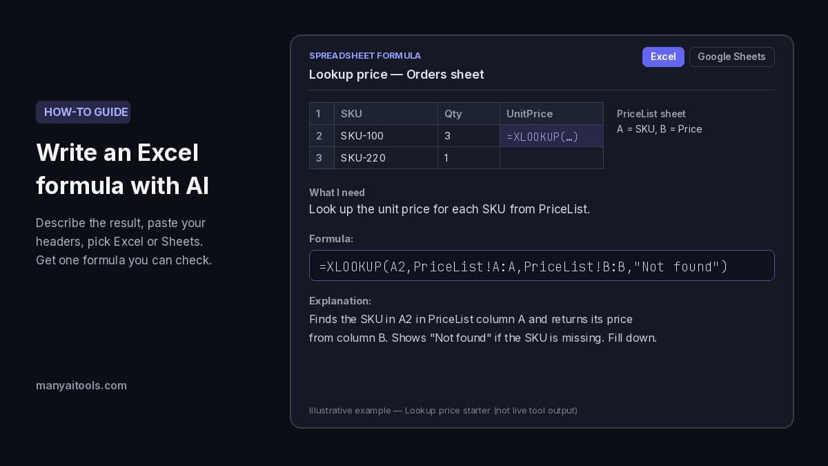
Example formula for the sample Lookup price request (illustrative, not live tool output).

To write an Excel formula with AI, describe the result you want in one plain sentence, paste your column headers and two or three sample rows, say whether you're in Excel or Google Sheets, and ask for one formula plus a short explanation. Then test it on a few rows before you fill it down. The headers and sample rows matter most: they let the AI use your real columns instead of guessing.

This guide covers when a formula is the right fix, how to describe what you need so the first answer works, the Excel vs Google Sheets differences that trip people up, and three worked examples (lookup, sum by category, and workdays) you can copy.

When you need a formula (and when you don't)

A formula is the right tool when the same calculation repeats on every row, or when a number has to update by itself as the data changes. Typical jobs:

• Look something up from another table: a price for a SKU, a manager for an employee ID, a region for a postcode.
• Total or count by a condition: spend per category, orders per customer, tickets still open.
• Clean or reshape data: a unique list of emails, first names split from full names, text trimmed of stray spaces.
• Work with dates: a due date 10 business days out, the number of days between two dates, the month of a timestamp.

If you only need an answer once ("what did we spend on travel last quarter?"), a filter or a pivot table may be faster. If you'll check it again next week, write the formula.

How to describe what you need

The best request has three parts: the goal, the layout, and the dialect.

1. The goal, in one sentence. Say what the cell should show, not which function you think you need. "Sum Amount for rows where Category matches F2" beats "I need a SUMIF".
2. The layout. List the headers with their column letters, the sheet names involved, and where the data starts and ends. Two or three sample rows help the AI spot dates stored as text, blank rows, or numbers with currency symbols.
3. The dialect. Excel or Google Sheets, and for Excel, whether it's Microsoft 365 or an older version like Excel 2016 or 2019. Several modern functions only exist in newer versions.

A good request looks like this:

What I need: Look up the unit price for each SKU in column A from a PriceList sheet that has SKU in column A and Price in column B. Return the price in column C of my Orders sheet.

Sheet layout: Orders headers: A=SKU, B=Qty, C=UnitPrice. PriceList headers: A=SKU, B=Price. Sample Orders rows: A2=SKU-100, B2=3; A3=SKU-220, B3=1.

Notice what's in there: real sheet names, real column letters, and the exact cell where the answer goes. That's everything a formula needs.

Don't let it invent sheet names or ranges

The most common reason an AI formula "doesn't work" is a reference to something that isn't in your file: a sheet called Data when yours is Sheet1, a named range that was never created, or a range like A1:A10 when your data runs to row 500.

• Name every sheet the formula touches, spelled exactly as it appears on the tab. Sheet names with spaces need single quotes in a formula: 'Price List'!A:B.
• Give the real range or say "data starts at row 2 and grows". Then you can choose between a fixed range (B2:B500) and a whole column (B:B).
• Check every reference in the answer against your sheet before you trust the result. If the formula mentions something you didn't give it, that's a placeholder to replace, not a feature.

Our helper is built around that rule: it uses only the headers and sheets you mention, and when you don't give ranges it uses obvious placeholders like A2:A100 and tells you what to adjust.

Excel vs Google Sheets: the gotchas

Most everyday formulas (SUM, SUMIF, IF, VLOOKUP, WORKDAY) work the same in both. These are the differences that cause errors when you copy a formula from one to the other.

• XLOOKUP needs a newer Excel. It's in Microsoft 365, Excel 2021 and later, and Excel for the web, and Google Sheets supports it too. In Excel 2019 or earlier, use VLOOKUP or INDEX/MATCH instead.
• Filling a whole column at once works differently. Excel 365 "spills" an array formula into the cells below on its own. Google Sheets needs ARRAYFORMULA for most functions to do the same, and ARRAYFORMULA doesn't exist in Excel.
• Open-ended ranges are Sheets-only. A2:A (row 2 to the bottom) is valid in Google Sheets but not in Excel. In Excel, use a fixed range like A2:A1000 or the whole column A:A.
• UNIQUE, FILTER and SORT need Excel 365 or Excel 2021 and later. They work in every version of Google Sheets. One more difference: Excel's UNIQUE ignores case, so "Ann@x.com" and "ann@x.com" count as one value, while Google Sheets treats them as two.
• Blocked results show different errors. If cells below a spilling formula aren't empty, Excel shows #SPILL! and Google Sheets shows #REF!. Clear the cells and it recalculates.
• Separators depend on your locale. In regions that use a comma for decimals, both apps use semicolons between arguments: =SUMIF(B:B;F2;D:D).

For example, to fill a whole UnitPrice column with one formula in C2, Excel 365 (or Excel 2021 and later) can spill a lookup down from a range and leave blank rows blank:

=IF(A2:A100="","",XLOOKUP(A2:A100,PriceList!A:A,PriceList!B:B,"Not found"))

The Google Sheets version wraps the same idea in ARRAYFORMULA and uses an open-ended range:

=ARRAYFORMULA(IF(A2:A="","",IFERROR(VLOOKUP(A2:A,PriceList!A:B,2,FALSE),"Not found")))

Both formulas need the cells below C2 to be empty. That's why choosing the right dialect up front matters: the same goal often needs a different formula.

How to write a formula with our free AI helper

Our Spreadsheet Formula Helper does this in one step. Here's the flow:

1. Describe what you need in plain language: the calculation, lookup, or cleanup.
2. Paste headers or sample rows (optional, but it's what makes the formula fit your sheet).
3. Choose Excel or Google Sheets. The answer follows that dialect and notes any function that only works in one of them.
4. Copy the formula, paste it into the first cell, and check it against a few rows you can verify by hand.
5. Adjust ranges and fill down once the first rows are right.

Every answer comes back as a Formula line and a short Explanation covering which cells it uses and any caveats. Not sure how to phrase it? Start from a sample: Lookup price, Sum by category, Unique list, or Workdays each loads a request and a sheet layout you can edit.

Sign in with Google to try it. New accounts get free starter credits, and credit packs from $5 are shared with our other writing and photo tools.

Worked example 1: Look up a price from another sheet

These inputs match the Lookup price starter on the tool page. The formulas in these examples were written for this guide to show the format, not copied from live tool output.

Request: Look up the unit price for each SKU in column A from the PriceList sheet (SKU in column A, Price in column B). Return it in column C of the Orders sheet.

Formula (Excel 365 / Google Sheets), in Orders!C2:

=XLOOKUP(A2,PriceList!A:A,PriceList!B:B,"Not found")

Explanation: Finds the SKU in A2 in PriceList column A and returns the matching price from column B. If the SKU isn't on the price list, the cell shows "Not found" instead of an error. Fill down from C2 for the other orders. On Excel 2019 or earlier, use =IFERROR(VLOOKUP(A2,PriceList!A:B,2,FALSE),"Not found") instead.

The FALSE in VLOOKUP means "exact match only". Leave it out and VLOOKUP assumes the list is sorted and may return the wrong price without warning. That's one of the most common lookup bugs, and a good thing to check in any formula you're given.

Worked example 2: Sum by category

These inputs match the Sum by category starter.

Request: Sum Amount for rows where Category equals the value in F2.

Sheet layout: A=Date, B=Category, C=Vendor, D=Amount. Sample rows: 2026-01-03, Travel, Uber, 24.50 and 2026-01-04, Software, Notion, 20. F2 holds the category to total, for example Travel.

Formula (Excel and Google Sheets):

=SUMIF(B:B,F2,D:D)

Explanation: Adds every Amount in column D where the Category in column B matches F2. With the sample rows and F2 set to Travel, the result is 24.50. Type a different category in F2 and the total updates. For two conditions (category and month, say), ask for SUMIFS instead.

If the total comes out as 0 when it clearly shouldn't, check whether the amounts are stored as text (often left-aligned, or pasted with a currency sign). SUMIF skips text, so convert the column to numbers first.

Worked example 3: Add business days to a date

These inputs match the Workdays starter.

Request: Given a start date in A2 and a number of business days in B2, return the end date, skipping weekends.

Sheet layout: A2 = 2026-03-02, B2 = 10.

Formula (Excel and Google Sheets):

=WORKDAY(A2,B2)

Explanation: Counts 10 working days forward from Monday, March 2, 2026, skipping Saturdays and Sundays, and returns Monday, March 16, 2026. To skip holidays too, list them in a range and add it as a third argument, for example =WORKDAY(A2,B2,H2:H10) with the holiday dates in H2:H10.

If the cell shows a number like 46097 instead of a date, the formula worked: spreadsheets store dates as numbers. Format the cell as a date. And if your weekend isn't Saturday and Sunday, ask for WORKDAY.INTL, which lets you choose the weekend days.

Before you fill it down

• Every sheet name and column in the formula matches your file.
• You chose the right dialect (Excel version or Google Sheets).
• You tested the first few rows against answers you can check by hand.
• Lookups use exact match (FALSE in VLOOKUP, or XLOOKUP's default).
• Numbers and dates are real numbers and dates, not text.
• Cells below a spilling or ARRAYFORMULA result are empty.

Quick answers

Can AI write Excel formulas? Yes, and it's good at it when you give it your real headers and sample rows. Describe the result you want, say whether you use Excel or Google Sheets, then test the formula on a few rows before you rely on it.

Is there a free AI Excel formula generator? Our Spreadsheet Formula Helper is free to try after Google sign-in, with starter credits like our other tools. If you need more, credit packs start at $5.

Does the same formula work in Google Sheets? Usually, for everyday functions like SUMIF, VLOOKUP and WORKDAY. Array formulas, open-ended ranges like A2:A, and newer functions like XLOOKUP and UNIQUE behave differently, so pick your dialect before you generate.

Why does my AI formula return an error? Most often it points at a sheet or range that doesn't exist in your file, uses a function your Excel version doesn't have, or tries to spill into cells that aren't empty. Check those three first.

Should I use VLOOKUP or XLOOKUP? Use XLOOKUP if everyone who opens the file has Excel 365, Excel 2021 or later, or Google Sheets. It's easier to read and defaults to an exact match. Use VLOOKUP with FALSE when the file has to work in older Excel.

Pulling data off websites to put in a sheet? An AI browser agent can collect it one row per item, ready to paste and work with.